Subproject
ArcadeDB
A multi-model database engine that keeps documents, graphs, vectors, and time series in one transactional engine, plus the Python package that runs that engine inside your process, benchmarked against the comparators in each category.
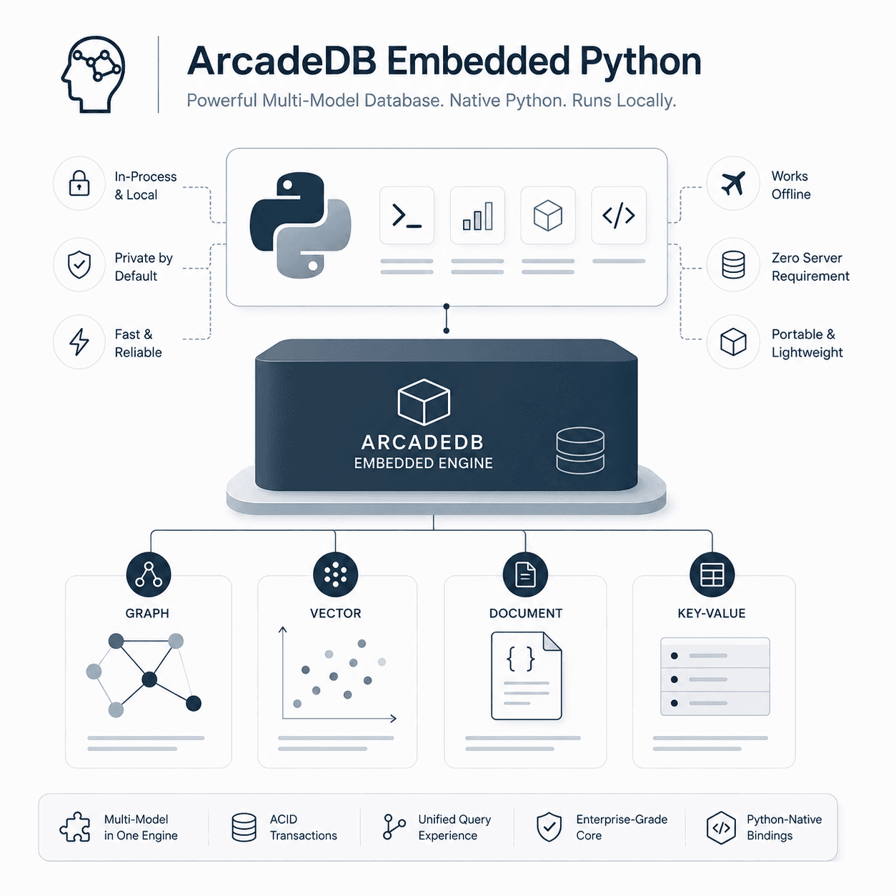
Engine
One storage engine for documents, graphs, vectors, and time series.
ArcadeDB is a Java engine. It runs embedded inside a Java process or as a server behind HTTP, Bolt, Postgres, and Redis protocols, and almost everyone runs the server. HumemAI wraps the same engine for Python through JPype, so it also runs inside a Python process; that package is the Python section further down. It answers SQL, in its own dialect, and Cypher, so the two industry-standard query languages and the skills and tools around them carry over; the other single-stack multi-model engines on this page each have a language of their own, SurrealQL, AQL, and MongoDB's query language. Every benchmark table on this page measures both deployments of the same build, which is what the Mode column means. Upstream also lists key-value and full-text search among its models; this page does not measure them.
Most databases that call themselves multi-model are several engines behind one API. ArcadeDB is not. Everything it stores sits on the same pages, goes through the same write-ahead log (WAL), and commits in the same transaction, so a write that touches a document, an edge, and a vector index is one ACID transaction (atomic, consistent, isolated, and durable) instead of three that have to be coordinated.
The indexes work the same way. LSM trees (log-structured merge trees), full-text, geo, hash, and both dense and sparse vector indexes all commit in the same transaction as the records they index. Replication follows from that: Raft ships page changes from the shared log, so every model replicates without replication code per model.
Vectors are the one exception. The vector records are transactional, logged, and replicated like everything else, but the nearest-neighbour graph used to search them is not: it is built in the background and can be rebuilt. The data is the source of truth and the search structure catches up to it. That is more than a standalone vector store offers, and less than a fully transactional index would be.
Benchmarks
One machine, fixed limits, one job at a time.
Every number on this page was measured on one machine: an Intel Core i9-12900HK (14 cores, 6 performance and 8 efficient, 20 threads, 24 MiB L3), 64 GiB of memory, a Samsung 980 PRO 2 TB NVMe drive, Ubuntu 26.04 with Docker. Each run is pinned to the twelve hardware threads of the six performance cores (cpuset 0-11) and to a memory cap that depends on the size: 8 GiB up to 100k documents, 16 GiB at 1M, 32 GiB at 20M rows, 36 GiB at ten million vectors, with a JVM (Java virtual machine) heap of half the cap for the Java engines, except at ten million vectors, where every Java engine runs 24 of the 36 GiB because the vector build fills it. One job runs at a time; a served engine and its client share the same cap. Every comparator is pinned by image digest, and the build measured is listed under each table.
The method behind these numbers is documented in full at docs.humem.ai/arcadedb, which covers the protocol, the answer checking that compares every engine's result rather than only its speed, how to run a lane yourself, and how this page is generated and gated. The conditions below hold for every table on this page. A table adds its own beneath its caption where they differ. Latency columns are p50 and p99, the median and the 99th percentile of the query times, in milliseconds.
- Every engine runs in Docker under an identical cpuset and memory cap, one job at a time, on the same host.
- Peak memory is the largest amount an engine held in its own address space, added over every container a run used, and it leaves out the file cache the kernel keeps on the engine's behalf. That is the right number for engines that manage their own memory, and an undercount for engines that lean on the kernel instead, so compare it down one engine's rows rather than across engines that work differently.
- Each printed cell is the median of 5 repetitions, with min and max carried alongside; nothing here is a single sample.
- Defaults first. Where a default would make the comparison meaningless, it is equalized and the override is disclosed rather than hidden.
- Comparators are pinned by sha256 image digest, not by a floating tag.
- A disk reading is taken after the queries, so it includes anything querying wrote; for a served row it is the server container alone, the client being only the driver. A server reading is taken once two samples agree within 1%, an embedded reading once on the stopped container. A blank disk cell is a row measured before the disk reading existed (2026-08-14). Neo4j's value includes the transaction-log files it preallocates in 256 MiB steps, which is how Neo4j uses disk; turning that off would have slowed its writes, so it stays on.
- Durability is at each engine's default, and the defaults differ: ArcadeDB does not flush its write-ahead log at commit (txWalFlush=0), PostgreSQL and Neo4j fsync at every commit, and SQLite is the one comparator not at its default: it runs in WAL mode with synchronous=NORMAL, the common production setting, because its default rollback journal fsyncs twice per commit. On the write rows (document OLTP, TPC-C new-order, graph writes, the cross-model transaction) ArcadeDB's lead over the fsyncing servers is largely this default plus the absence of a network hop, not the engine. The next campaign matches every engine at the relaxed end instead: each one commits without waiting for the disk, which is what SQLite's setting above already means. Three engines have no setting for it, Neo4j, DuckDB, and LadybugDB, each measured rather than assumed, and each is named on the tables it appears on.
Benchmarks
Document OLTP and OLAP on TPC.
Most people arrive with tables. ArcadeDB stores them as documents and answers the same SQL, so documents come first. Every engine below answers the same questions in its own language: SQL where it has one, MongoDB's aggregation pipeline, SurrealQL for SurrealDB. The benchmarks are TPC-C and TPC-H, the long-standing transaction and analytics benchmarks. TPC-C is OLTP, online transaction processing: many small reads and writes. TPC-H is OLAP, online analytical processing: a few large scanning queries. Both run at SF1, where SF is the scale factor, the size of the generated data set.
TPC-C's new-order transaction (read a part, insert an order line, update stock) on the TPC-H tables, against DuckDB and PostgreSQL. PostgreSQL appears twice, at its image defaults and tuned with its buffer and work memory fitted to the container.
| Engine | Mode | Size | new-order p50 ms ↓ | new-order p99 ms ↓ | OLTP ops/s ↑ | ingest documents/s ↑ | ingest total s ↓ | peak memory GiB ↓ | disk GiB ↓ |
|---|---|---|---|---|---|---|---|---|---|
| ArcadeDB | embedded | TPC-H SF1 (6.0M line items) | 0.40 | 0.80 | 2,073 | 41k | 150.9 | 6.64 | 0.62 |
| ArcadeDB | server | TPC-H SF1 (6.0M line items) | 1.15 | 2.06 | 819 | 32k | 192.9 | 9.22 | 0.65 |
| ArangoDB | server | TPC-H SF1 (6.0M line items) | 2.65 | 3.86 | 363 | 95k | 65.1 | 4.28 | 1.02 |
| DuckDB | embedded | TPC-H SF1 (6.0M line items) | 9.66 | 18.6 | 99 | 2.46M | 2.52 | 3.36 | 0.071 |
| MongoDB | server | TPC-H SF1 (6.0M line items) | 6.95 | 17.1 | 137 | 123k | 50.3 | 7.13 | 0.77 |
| PostgreSQL | server | TPC-H SF1 (6.0M line items) | 2.39 | 5 | 319 | 364k | 17.1 | 3.35 | 0.79 |
| SQLite | embedded | TPC-H SF1 (6.0M line items) | 0.011 | 0.019 | 20k | 334k | 18.6 | 3.36 | 0.39 |
| SurrealDB | embedded | TPC-H SF1 (6.0M line items) | 0.14 | 0.21 | 6,985 | 11k | 550.6 | 7.33 | 2.51 |
| SurrealDB | server | TPC-H SF1 (6.0M line items) | 10.1 | 19.3 | 90 | 22k | 283.3 | 8.89 | 0.67 |
↑ higher is better, ↓ lower is better; the best value in each column, within one size, is bold
Measured rows: benchmarks/experiments/results/runs_paper.csv
Exact builds measured
- arcadedb 26.9.1-dev · 8d6af9475 (in-process)
- arcadedb 26.9.1-dev · 8d6af9475
arcadedb-c25:8d6af9475 - arangodb 3.12.11
arangodb@563cb2c07af0… - duckdb 1.5.5
- mongodb 8.2.12
mongo@41afd6e1183f… - postgresql 17.10
postgres@de1e13ca9437… - sqlite 3.46.1
- surrealdb 2.3.10
- surrealdb 3.2.4
surrealdb/surrealdb@6a5002363ff5…
- Q1 and Q6 are TPC-H's own query numbers. Q1 groups and aggregates the whole line-item table, so it measures a full scan; Q6 sums one column under a narrow filter, so it measures how well an engine skips what it does not need.
- New-order is TPC-C's checkout transaction: it reads a customer and a warehouse, inserts an order with its line items, and updates stock, all in one transaction.
- Disk is what the workload left on disk, in GiB: the engine's writable layer plus its volumes after the cell, minus the same engine's empty footprint.
- The two SurrealDB rows are not one engine in two deployments. The embedded arm runs the core its Python driver carries and the served arm runs the released server, and here those are surrealdb 2.3.10 and surrealdb 3.2.4 -- different versions on different storage engines, released about a year apart. Read each row against the other engines on the table rather than against each other: the distance between these two is not the cost of a network hop.
- ArcadeDB (embedded) and ArcadeDB (server) run on a JVM, and for them this column is close to the heap they were given rather than the memory the work needed: ArcadeDB (server)'s 9.22 GiB here is about 115 per cent of its 8g heap, and across every heap this page has run the peak lands between about two thirds of the heap and a fifth above it. Every engine on a table gets the same memory envelope; how much of it a JVM takes is a property of the runtime, so read these cells against each other rather than against an engine that manages its own memory.
- PostgreSQL's memory cell is not comparable to the others: this column counts memory an engine holds in its own address space, and PostgreSQL holds its data in shared memory and the kernel's file cache instead. At TPC-H SF1 (6.0M line items), of the 3.35 GiB shown, 3.344 GiB is our Python client and 0.008 GiB is the database.
- Each repetition runs 1,000 new-order transactions; the p50 and p99 are over those, and OLTP ops/s is their rate.
TPC-H Q1 (scan every line item, group, and sum) and Q6 (filter a date range, sum one column) on the same documents. This is the workload ArcadeDB loses by the widest margin on the page.
| Engine | Mode | Size | Q1 p50 ms ↓ | Q1 p99 ms ↓ | Q6 p50 ms ↓ | Q6 p99 ms ↓ | ingest documents/s ↑ | ingest total s ↓ | peak memory GiB ↓ | disk GiB ↓ |
|---|---|---|---|---|---|---|---|---|---|---|
| ArangoDB | server | TPC-H SF1 (6.0M line items) | 12k | 13k | 1,764 | 1,773 | 95k | 65.1 | 4.28 | 1.02 |
| DuckDB | embedded | TPC-H SF1 (6.0M line items) | 15.5 | 16.9 | 7.23 | 8.69 | 2.46M | 2.52 | 3.36 | 0.071 |
| MongoDB | server | TPC-H SF1 (6.0M line items) | 9,815 | 9,938 | 1,139 | 1,270 | 123k | 50.3 | 7.13 | 0.77 |
| PostgreSQL | server | TPC-H SF1 (6.0M line items) | 330.7 | 1,074 | 105.8 | 109.6 | 364k | 17.1 | 3.35 | 0.79 |
| SQLite | embedded | TPC-H SF1 (6.0M line items) | 9,233 | 9,268 | 1,027 | 1,033 | 334k | 18.6 | 3.36 | 0.39 |
| SurrealDB | embedded | TPC-H SF1 (6.0M line items) | 102k | 104k | 11k | 11k | 11k | 550.6 | 7.33 | 2.51 |
| SurrealDB | server | TPC-H SF1 (6.0M line items) | 55k | 55k | 5,377 | 5,563 | 22k | 283.3 | 8.89 | 0.67 |
↑ higher is better, ↓ lower is better; the best value in each column, within one size, is bold
Measured rows: benchmarks/experiments/results/runs_paper.csv
Exact builds measured
- arangodb 3.12.11
arangodb@563cb2c07af0… - duckdb 1.5.5
- mongodb 8.2.12
mongo@41afd6e1183f… - postgresql 17.10
postgres@de1e13ca9437… - sqlite 3.46.1
- surrealdb 2.3.10
- surrealdb 3.2.4
surrealdb/surrealdb@6a5002363ff5…
- Q1 and Q6 are TPC-H's own query numbers. Q1 groups and aggregates the whole line-item table, so it measures a full scan; Q6 sums one column under a narrow filter, so it measures how well an engine skips what it does not need.
- New-order is TPC-C's checkout transaction: it reads a customer and a warehouse, inserts an order with its line items, and updates stock, all in one transaction.
- ArcadeDB has no row on this table. Answer checking built for the next campaign found that the two queries it ran here were not the questions the comparators answered: one of the five aggregates was missing from our Q1 text, and its Q6 excluded the boundary discount because the engine reads `>= 0.05` against a decimal literal as strictly greater. Both errors made its numbers faster than the truth, so they are withdrawn rather than shown with a caveat, and the next the real run measures them with every engine's answer compared.
- Disk is what the workload left on disk, in GiB: the engine's writable layer plus its volumes after the cell, minus the same engine's empty footprint.
- The two SurrealDB rows are not one engine in two deployments. The embedded arm runs the core its Python driver carries and the served arm runs the released server, and here those are surrealdb 2.3.10 and surrealdb 3.2.4 -- different versions on different storage engines, released about a year apart. Read each row against the other engines on the table rather than against each other: the distance between these two is not the cost of a network hop.
- PostgreSQL's memory cell is not comparable to the others: this column counts memory an engine holds in its own address space, and PostgreSQL holds its data in shared memory and the kernel's file cache instead. At TPC-H SF1 (6.0M line items), of the 3.35 GiB shown, 3.344 GiB is our Python client and 0.008 GiB is the database.
- Each repetition runs every query 100 times; the p50 and p99 are over those runs.
- Indexes on this table are matched by effect rather than by rule: ArcadeDB (embedded), ArcadeDB (server), MongoDB, PostgreSQL, PostgreSQL (tuned), SurrealDB (embedded) and SurrealDB (server) build one; ArangoDB, DuckDB and SQLite build none, because measuring it showed the index costs them or changes nothing. Where building one was a choice, the engine was timed with it and without it and the faster configuration kept; where an engine reaches these queries through its own primary key or record id, that is its equivalent. The time an index took to build is the index column.
- ArangoDB, MongoDB and SQLite at TPC-H SF10 (60.0M line items): the analytics cell exceeded its 2 hour budget, the same budget every engine on this table had, on its first attempt and was not retried; there is no row.
- SurrealDB (embedded) at TPC-H SF10 (60.0M line items): the analytics cell reached the 32g memory envelope (peak 32,768 MiB) and was killed by the kernel, the same envelope every engine on this table had; it did not run out of time, and there is no row.
- SurrealDB (server) at TPC-H SF10 (60.0M line items): the analytics cell failed inside its budget and was not retried, so there is no row. What it reported: websockets.exceptions.ConnectionClosedError: no close frame received or sent
Benchmarks
Graph OLTP and OLAP on LDBC.
Graph is what most people use ArcadeDB for. The benchmark is LDBC-SNB, the Linked Data Benchmark Council's Social Network Benchmark, a synthetic social network at two scale factors, SF1 and SF10. ArcadeDB, Neo4j, and LadybugDB answer the queries in Cypher, the most common graph query language; SurrealDB answers the same queries in SurrealQL. Neo4j is the most widely used graph database, so it is the comparator. LadybugDB is here because it is embedded and columnar, the closest comparator to running ArcadeDB inside your own process.
ArcadeDB embedded answers all four queries faster than Neo4j at both sizes. That is the strongest head-to-head result on this page.
Graph OLTP against Neo4j and LadybugDB on LDBC-SNB. Point is a single vertex lookup, 1-hop and 2-hop walk that many edges out from a starting person, and write inserts one edge.
| Engine | Mode | Size | point p50 ms ↓ | point p99 ms ↓ | 1-hop p50 ms ↓ | 1-hop p99 ms ↓ | 2-hop p50 ms ↓ | 2-hop p99 ms ↓ | write p50 ms ↓ | write p99 ms ↓ | ingest vertices+edges/s ↑ | ingest total s ↓ | peak memory GiB ↓ | disk GiB ↓ |
|---|---|---|---|---|---|---|---|---|---|---|---|---|---|---|
| ArcadeDB | embedded | SF1 (10k people, 181k friendships) | 0.49 | 0.95 | 0.45 | 1.19 | 0.70 | 6.42 | 0.56 | 0.85 | 89k | 2.13 | 1.75 | 0.012 |
| ArcadeDB | server | SF1 (10k people, 181k friendships) | 1.24 | 2.28 | 1.20 | 2.13 | 1.49 | 7.40 | 1.34 | 1.83 | 26k | 7.45 | 3.33 | 0.068 |
| ArangoDB | server | SF1 (10k people, 181k friendships) | 0.81 | 1.13 | 0.98 | 1.44 | 2.31 | 16.3 | 0.81 | 1.08 | 98k | 1.94 | 0.29 | 0.047 |
| DuckPGQ | embedded | SF1 (10k people, 181k friendships) | 0.25 | 0.30 | 0.93 | 1.21 | 2.24 | 3.72 | 10.5 | 16.7 | 203k | 0.94 | 0.14 | 0.036 |
| FalkorDB | server | SF1 (10k people, 181k friendships) | 0.13 | 0.29 | 0.21 | 0.47 | 0.38 | 1.02 | 0.18 | 0.41 | 41k | 4.69 | 0.17 | 0 |
| LadybugDB | embedded | SF1 (10k people, 181k friendships) | 0.16 | 0.25 | 1.05 | 1.27 | 4.04 | 4.71 | 9.82 | 19.2 | 389k | 0.49 | 0.22 | 0.0055 |
| Memgraph | server | SF1 (10k people, 181k friendships) | 0.14 | 0.27 | 0.15 | 0.27 | 0.20 | 0.76 | 0.15 | 0.25 | 74k | 2.59 | 0.46 | 0.023 |
| Neo4j | server | SF1 (10k people, 181k friendships) | 6.16 | 12.0 | 5.73 | 9.29 | 4.75 | 7.22 | 7.59 | 19.4 | 37k | 5.13 | 4.69 | 0.015 |
| SurrealDB | embedded | SF1 (10k people, 181k friendships) | 0.044 | 0.050 | 0.70 | 9.46 | 14.9 | 185.6 | 0.16 | 0.19 | 14k | 13.6 | 0.56 | 0.10 |
| SurrealDB | server | SF1 (10k people, 181k friendships) | 0.11 | 0.30 | 0.19 | 0.57 | 0.50 | 3.05 | 17.6 | 32.3 | 20k | 9.51 | 0.31 | 0.047 |
| ArcadeDB | embedded | SF10 (66k people, 1.9M friendships) | 0.50 | 1.03 | 0.61 | 1.40 | 1.67 | 17.5 | 0.66 | 0.92 | 88k | 22.9 | 8.05 | 0.13 |
| ArcadeDB | server | SF10 (66k people, 1.9M friendships) | 1.19 | 1.76 | 1.35 | 2.19 | 2.50 | 19.0 | 1.41 | 1.81 | 28k | 71.4 | 7.93 | 0.16 |
| ArangoDB | server | SF10 (66k people, 1.9M friendships) | 0.85 | 1.19 | 1.05 | 2.06 | 5.82 | 73.8 | 0.93 | 1.17 | 92k | 21.8 | 0.78 | 0.88 |
| DuckPGQ | embedded | SF10 (66k people, 1.9M friendships) | 0.26 | 0.32 | 1.34 | 1.65 | 4.26 | 9.39 | 10.6 | 17.9 | 299k | 6.70 | 0.27 | 0.094 |
| FalkorDB | server | SF10 (66k people, 1.9M friendships) | 0.12 | 0.52 | 0.23 | 0.47 | 0.74 | 2.68 | 0.18 | 0.38 | 23k | 86.5 | 0.35 | 0 |
| LadybugDB | embedded | SF10 (66k people, 1.9M friendships) | 0.17 | 0.38 | 1.66 | 4.16 | 5.55 | 10.9 | 9.77 | 11.7 | 543k | 3.69 | 0.37 | 0.052 |
| Memgraph | server | SF10 (66k people, 1.9M friendships) | 0.14 | 0.31 | 0.15 | 0.24 | 0.30 | 2.28 | 0.15 | 0.25 | 72k | 27.8 | 0.63 | 0.24 |
| Neo4j | server | SF10 (66k people, 1.9M friendships) | 7.40 | 12.5 | 7.03 | 9.97 | 6.31 | 10.5 | 8.52 | 14.3 | 44k | 45.0 | 13.0 | 0.66 |
| SurrealDB | embedded | SF10 (66k people, 1.9M friendships) | 0.046 | 0.054 | 1.20 | 24.0 | 59.4 | 800.4 | 0.18 | 0.20 | 11k | 175.3 | 5.06 | 1.09 |
| SurrealDB | server | SF10 (66k people, 1.9M friendships) | 0.17 | 0.67 | 0.41 | 1.44 | 1.22 | 13.8 | 17.6 | 29.7 | 18k | 112.4 | 2.02 | 0.26 |
↑ higher is better, ↓ lower is better; the best value in each column, within one size, is bold
Measured rows: benchmarks/experiments/results/runs_paper.csv
Exact builds measured
- arcadedb 26.9.1-dev · 8d6af9475 (in-process)
- arcadedb 26.9.1-dev · 8d6af9475
arcadedb-c25:8d6af9475 - arangodb 3.12.11
arangodb@563cb2c07af0… - duckpgq 1.5.4
- falkordb 4.20.6
falkordb/falkordb@0a9fe4d1ee0b… - ladybugdb 0.19.1
- memgraph 3.13.1
memgraph/memgraph@4710bee1ab5b… - neo4j 2026.07.1
neo4j@1ee8f6fa220f… - surrealdb 2.3.10
- surrealdb 3.2.4
surrealdb/surrealdb@6a5002363ff5…
- Every engine traverses the same persons-and-KNOWS projection, with edges stored in both directions.
- Disk is what the workload left on disk, in GiB: the engine's writable layer plus its volumes after the cell, minus the same engine's empty footprint.
- The two SurrealDB rows are not one engine in two deployments. The embedded arm runs the core its Python driver carries and the served arm runs the released server, and here those are surrealdb 2.3.10 and surrealdb 3.2.4 -- different versions on different storage engines, released about a year apart. Read each row against the other engines on the table rather than against each other: the distance between these two is not the cost of a network hop.
- ArcadeDB (embedded), ArcadeDB (server) and Neo4j run on a JVM, and for them this column is close to the heap they were given rather than the memory the work needed: Neo4j's 4.69 GiB here is about 117 per cent of its 4g heap, and across every heap this page has run the peak lands between about two thirds of the heap and a fifth above it. Every engine on a table gets the same memory envelope; how much of it a JVM takes is a property of the runtime, so read these cells against each other rather than against an engine that manages its own memory.
- Each repetition runs every read against a fresh set of start persons (SF1 (10k people, 181k friendships): 500, SF10 (66k people, 1.9M friendships): 200); the p50 and p99 are over those.
- FalkorDB at SF1 (10k people, 181k friendships) and SF10 (66k people, 1.9M friendships): its disk cells are 0.0 because the server container did not grow over its empty footprint during the run; read them as a floor under 0.01 GiB, not as a size.
- Ingest paths: ArcadeDB embedded loads through the Java API (newVertex, newEdge) in 5,000-record transactions; served sends CREATE VERTEX and CREATE EDGE statements as sqlscript batches over HTTP; Neo4j and Memgraph UNWIND batches over bolt; FalkorDB the same UNWIND batches over the Redis protocol; LadybugDB COPY from CSV, its native bulk path; DuckPGQ Arrow INSERT SELECT into the persons and knows tables under a property graph.
Graph OLAP, queries over the whole graph, is a different job from single traversals, and ArcadeDB has a separate mechanism for it. A Graph Analytical View (GAV) is an in-memory copy of the graph, built once, that the planner uses for queries touching most of the vertices. It is optional, so the table below carries the same engine twice, with the view and without it, and the cost of building the view is measured rather than assumed.
At SF10 the view is worth 6.9x on top degree and about 2.6x on the other two, which is enough to move ArcadeDB from behind Neo4j to ahead of it on all three. LadybugDB wins all three regardless, because it stores the graph in columns, the same reason DuckDB wins the analytical queries above.
| Engine | Mode | Size | average friend age p50 ms ↓ | average friend age p99 ms ↓ | friends in same city p50 ms ↓ | friends in same city p99 ms ↓ | most friends p50 ms ↓ | most friends p99 ms ↓ | view build s ↓ | ingest vertices+edges/s ↑ | ingest total s ↓ | peak memory GiB ↓ | disk GiB ↓ |
|---|---|---|---|---|---|---|---|---|---|---|---|---|---|
| ArcadeDB | embedded | SF1 (10k people, 181k friendships) | 110.5 | 118.4 | 107.4 | 118.7 | 37.5 | 63.4 | — | 88k | 2.16 | 2.70 | 0.012 |
| ArcadeDB (GAV) | embedded | SF1 (10k people, 181k friendships) | 42.8 | 53.9 | 40.6 | 70.0 | 9.77 | 17.8 | 1.05 | 60k | 3.18 | 2.70 | 0.015 |
| ArcadeDB | server | SF1 (10k people, 181k friendships) | 116.5 | 123.6 | 115.7 | 122.7 | 38.4 | 48.3 | — | 25k | 7.57 | 3.33 | 0.068 |
| ArcadeDB (GAV) | server | SF1 (10k people, 181k friendships) | 45.4 | 55.0 | 43.0 | 48.7 | 8.22 | 17.1 | 1.04 | 22k | 8.53 | 3.34 | 0.068 |
| ArangoDB | server | SF1 (10k people, 181k friendships) | 532.1 | 547.2 | 544.2 | 571.3 | 45.4 | 48.2 | — | 98k | 1.95 | 0.52 | 0.047 |
| LadybugDB | embedded | SF1 (10k people, 181k friendships) | 9.13 | 10.3 | 9.82 | 10.9 | 0.86 | 1.45 | — | 405k | 0.47 | 0.22 | 0.0045 |
| Neo4j | server | SF1 (10k people, 181k friendships) | 54.5 | 64.1 | 55.9 | 64.1 | 31.4 | 47.1 | — | 37k | 5.10 | 4.61 | 0.014 |
| SurrealDB | embedded | SF1 (10k people, 181k friendships) | 2,578 | 2,599 | 2,245 | 2,266 | 1,337 | 1,540 | — | 14k | 13.8 | 0.57 | 0.10 |
| SurrealDB | server | SF1 (10k people, 181k friendships) | 700.1 | 712.2 | 697.0 | 705.2 | 104.1 | 105.8 | — | 20k | 9.68 | 0.31 | 0.047 |
| ArcadeDB | embedded | SF10 (66k people, 1.9M friendships) | 1,201 | 1,211 | 1,171 | 1,191 | 361.9 | 375.7 | — | 88k | 22.9 | 8.11 | 0.13 |
| ArcadeDB (GAV) | embedded | SF10 (66k people, 1.9M friendships) | 461.1 | 468.9 | 440.2 | 465.4 | 52.4 | 61.5 | 2.06 | 80k | 25.0 | 8.19 | 0.16 |
| ArcadeDB | server | SF10 (66k people, 1.9M friendships) | 1,191 | 1,211 | 1,195 | 1,219 | 349.8 | 363.0 | — | 28k | 70.9 | 7.98 | 0.17 |
| ArcadeDB (GAV) | server | SF10 (66k people, 1.9M friendships) | 469.2 | 478.1 | 453.1 | 472.4 | 56.8 | 65.6 | 2.04 | 27k | 73.0 | 8.06 | 0.18 |
| ArangoDB | server | SF10 (66k people, 1.9M friendships) | 7,853 | 7,947 | 8,193 | 8,300 | 427.5 | 439.9 | — | 91k | 21.9 | 0.78 | 0.41 |
| LadybugDB | embedded | SF10 (66k people, 1.9M friendships) | 54.4 | 57.8 | 61.9 | 63.5 | 2.69 | 3.18 | — | 546k | 3.67 | 0.35 | 0.030 |
| Neo4j | server | SF10 (66k people, 1.9M friendships) | 630.9 | 643.9 | 816.5 | 833.7 | 328.7 | 344.4 | — | 44k | 45.4 | 13.0 | 0.66 |
| SurrealDB | embedded | SF10 (66k people, 1.9M friendships) | >2h | >2h | >2h | >2h | >2h | >2h | >2h | >2h | >2h | >2h | >2h |
| SurrealDB | server | SF10 (66k people, 1.9M friendships) | 7,834 | 7,950 | 7,931 | 8,006 | 942.4 | 956.8 | — | 18k | 112.8 | 2.14 | 0.26 |
↑ higher is better, ↓ lower is better; the best value in each column, within one size, is bold
Measured rows: benchmarks/experiments/results/runs_paper.csv
Exact builds measured
- arcadedb 26.9.1-dev · 8d6af9475 (in-process)
- arcadedb 26.9.1-dev · 8d6af9475
arcadedb-c25:8d6af9475 - arangodb 3.12.11
arangodb@563cb2c07af0… - ladybugdb 0.19.1
- neo4j 2026.07.1
neo4j@1ee8f6fa220f… - surrealdb 2.3.10
- surrealdb 3.2.4
surrealdb/surrealdb@6a5002363ff5…
- Three questions, each asked of the whole graph. Average friend age: for every city, the average age of the friends of the people who live there. Friends in same city: how many friendships connect two people in the same city. Most friends: which people have the highest number of friends. All three times are milliseconds.
- The two rows labelled ArcadeDB (embedded) are the same engine on the same data, differing only in whether that view is built. Both return identical answers.
- The benefit is uneven, and the three queries show why. Top degree gains most because it only walks adjacency. The other two read a property from the far end of every edge traversed, and that lookup costs the same either way, so it comes to dominate once the traversal itself is cheap.
- Disk is what the workload left on disk, in GiB: the engine's writable layer plus its volumes after the cell, minus the same engine's empty footprint.
- The two SurrealDB rows are not one engine in two deployments. The embedded arm runs the core its Python driver carries and the served arm runs the released server, and here those are surrealdb 2.3.10 and surrealdb 3.2.4 -- different versions on different storage engines, released about a year apart. Read each row against the other engines on the table rather than against each other: the distance between these two is not the cost of a network hop.
- ArcadeDB (embedded), ArcadeDB (embedded, GAV), ArcadeDB (server), ArcadeDB (server, GAV) and Neo4j run on a JVM, and for them this column is close to the heap they were given rather than the memory the work needed: Neo4j's 4.61 GiB here is about 115 per cent of its 4g heap, and across every heap this page has run the peak lands between about two thirds of the heap and a fifth above it. Every engine on a table gets the same memory envelope; how much of it a JVM takes is a property of the runtime, so read these cells against each other rather than against an engine that manages its own memory.
- The Graph Analytical View is a copy of the graph that ArcadeDB builds in memory, laid out for questions that sweep the whole graph rather than follow a few links. Building it took 2.1 seconds here at SF10 (66k people, 1.9M friendships), once, before any query was timed.
- Each repetition runs every query 100 times; the p50 and p99 are over those runs.
- SurrealDB (embedded) at SF10 (66k people, 1.9M friendships): the analytics cell exceeded its 2 hour budget, the same budget every engine on this table had, on its first attempt and was not retried; there is no row.
- In the cells: `>2h` means the cell ran past its tier's cap and was not retried. A dash is an operation the engine cannot express, never a slow one.
- Ingest paths: ArcadeDB embedded loads through the Java API (newVertex, newEdge) in 5,000-record transactions; served sends CREATE VERTEX and CREATE EDGE statements as sqlscript batches over HTTP; Neo4j and Memgraph UNWIND batches over bolt; FalkorDB the same UNWIND batches over the Redis protocol; LadybugDB COPY from CSV, its native bulk path; DuckPGQ Arrow INSERT SELECT into the persons and knows tables under a property graph.
Benchmarks
Vector search, dense and sparse.
Vector search is the newest of these models and the one with the most comparators, so it gets the most detail: three corpora, two kinds of vector, and recall reported beside every latency. It is also a workload ArcadeDB does not win, and the tables show that. Every engine on the dense table today indexes with HNSW (Hierarchical Navigable Small World), a graph of near neighbours that a query walks; an engine with a different index says so in the table's notes. Every corpus below is real and published, not generated, which matters most for sparse search.
A SPLADE (Sparse Lexical And Expansion model) vector stores one weight per word in the vocabulary, and nearly every weight is zero, so a search only has to look at the few words a query uses. Those words cost very different amounts. A common word has to be checked against a huge number of documents; a rare one against almost none.
Real writing has a few words that appear everywhere and a long tail that appear almost nowhere, so some queries are far more expensive than others. Generated data spreads words out evenly, which removes the expensive case and makes any approximate index look better than it is. Dense search uses published image descriptors for the same reason.
| Corpus | Vectors | Dimensions | Used for |
|---|---|---|---|
| SPLADE over MS MARCO | 100k, 1M, 8.84M | 30,109 | every sparse row |
| SIFT | 1M | 128 | the smaller dense size |
| DEEP | 9.99M | 96 | the ten-million dense size |
MS MARCO is a public search-relevance corpus, and the sparse vectors come from Big-ANN, a benchmark challenge for approximate nearest-neighbour search. SIFT and DEEP are standard image-descriptor sets.
Two of those sizes are ceilings, not choices. 8.84 million is the entire Big-ANN sparse base set, so no larger sparse size exists, and DEEP's 9.99 million is the ten-million slice that ships with exact ground truth. The dense corpora are also narrow beside a modern text embedding, which runs 768 to 3072 numbers wide against SIFT's 128 and DEEP's 96. That width is fixed by how the descriptors were produced, and these sets are used anyway because they publish exact nearest neighbours at ten million vectors, which is what makes recall comparable across engines. It does mean the dense rows describe index behaviour at 96 and 128 dimensions, and a 1536-dimension embedding is a different question.
The index settings are matched rather than left to each vendor's defaults. Dense search builds HNSW at ef_construction 100 and queries at ef_search 100 everywhere, with a graph degree of 16 neighbours per node. ArcadeDB spells that maxConnections 32, because its bound is per layer while hnswlib-style engines double theirs at the base layer, so matching the number instead of the degree would have given ArcadeDB twice the graph. Sparse search has no equivalent setting, so every engine runs its own defaults there and each table states what precision the index stores. Every query asks for the top 10, and recall@10 is the share of those 10 that are true nearest neighbours; the 10 is the k in recall@k.
Recall is reported next to every latency. A vector benchmark without a quality number is not a comparison, since any engine can be made faster by searching less thoroughly, and the engines here sit at different points on that trade.
Every engine in every table below runs under the same limits, one at a time on one machine, and each cell is the median of five repetitions. The exact build measured sits under each table. Two words recur: cold is the first timed pass after the index is built, and warm is a second pass over the same queries.
Every engine gets a settle step before any query is timed, the one-off operation that leaves it answering from a finished index rather than a half-built one: Elasticsearch refreshes and force-merges to a single segment, Milvus flushes and loads, Qdrant waits until the collection reports green, and ArcadeDB compacts its LSM segments.
Each comparator's sparse precision is read from its own documentation and source at the version measured. Qdrant and Milvus keep sparse weights at full 32-bit precision. Elasticsearch keeps about 9 significant bits, which its documentation puts at roughly 0.4% relative error, the lossiest of the engines here. ArcadeDB stores int8 posting weights by default and can store fp32; both are measured.
Sparse search on real SPLADE vectors against Elasticsearch, Milvus, and Qdrant. ArcadeDB appears four times, in both deployments and at both precisions: int8 posting weights are its default and fp32 is the ablation.
| Engine | Mode | Precision | Size | cold p50 ms ↓ | cold p99 ms ↓ | warm p50 ms ↓ | warm p99 ms ↓ | gain ↑ | recall@10 ↑ | ingest+index vectors/s ↑ | ingest+index total s ↓ | peak memory GiB ↓ | disk GiB ↓ |
|---|---|---|---|---|---|---|---|---|---|---|---|---|---|
| ArcadeDB | embedded | int8 | 100k vectors | 4.05 | 9.51 | 3.67 | 8.21 | 1.11x | 0.99 | 11k | 9.24 | 3.00 | 0.15 |
| ArcadeDB | embedded | fp32 | 100k vectors | 3.97 | 10.4 | 3.70 | 7.96 | 1.20x | 1 | 11k | 8.71 | 3.15 | 0.19 |
| ArcadeDB | server | int8 | 100k vectors | 4.93 | 12.0 | 4.49 | 8.84 | 1.17x | 0.99 | 3,957 | 25.3 | 4.36 | 0.19 |
| ArcadeDB | server | fp32 | 100k vectors | 5.02 | 10.7 | 4.32 | 8.35 | 1.21x | 1 | 3,863 | 25.9 | 4.37 | 0.23 |
| Elasticsearch | server | ~9-bit | 100k vectors | 3.42 | 6.87 | 2.82 | 4.59 | 1.31x | 1.00 | 2,869 | 34.9 | 4.78 | 0.094 |
| Milvus | server | fp32 | 100k vectors | 3.01 | 7.68 | 2.95 | 7.66 | 1.03x | 1 | 5,539 | 18.1 | 1.32 | 0.27 |
| pgvector | server | fp32 | 100k vectors | 1.01 | 1.80 | 0.84 | 1.59 | 1.20x | 0.82 | 1,519 | 65.8 | 0.14 | 0.46 |
| Qdrant | server | fp32 | 100k vectors | 0.88 | 1.31 | 0.89 | 1.12 | 0.98x | 1 | 12k | 8.44 | 0.69 | 0.25 |
| ArcadeDB | embedded | int8 | 1M vectors | 11.4 | 36.5 | 11.0 | 35.7 | 1.09x | 0.99 | 11k | 94.5 | 8.36 | 1.48 |
| ArcadeDB | embedded | fp32 | 1M vectors | 11.4 | 35.8 | 11.1 | 35.3 | 1.08x | 1 | 11k | 94.5 | 8.42 | 1.83 |
| ArcadeDB | server | int8 | 1M vectors | 12.9 | 39.7 | 12.1 | 36.9 | 1.14x | 0.99 | 4,023 | 248.6 | 8.62 | 1.50 |
| ArcadeDB | server | fp32 | 1M vectors | 12.8 | 39.1 | 11.8 | 36.7 | 1.15x | 1 | 3,967 | 252.1 | 8.65 | 1.86 |
| Elasticsearch | server | ~9-bit | 1M vectors | 10.0 | 21.6 | 9.08 | 20.6 | 1.14x | 1.00 | 2,981 | 335.5 | 9.05 | 0.90 |
| Milvus | server | fp32 | 1M vectors | 9.40 | 36.7 | 11.1 | 40.9 | 0.75x | 1 | 8,331 | 120.0 | 5.53 | 4.56 |
| pgvector | server | fp32 | 1M vectors | 1.30 | 2.59 | 1.25 | 2.55 | 1.06x | 0.77 | 1,498 | 667.5 | 0.31 | 3.62 |
| Qdrant | server | fp32 | 1M vectors | 2.85 | 4.15 | 2.87 | 4.20 | 0.99x | 1 | 11k | 94.8 | 2.27 | 1.45 |
| ArcadeDB | embedded | int8 | 8.84M vectors | 86.1 | 307.5 | 84.4 | 303.6 | 1.04x | 0.99 | 9,614 | 919.7 | 16.8 | 13.1 |
| ArcadeDB | embedded | fp32 | 8.84M vectors | 86.8 | 320.9 | 85.2 | 314.1 | 1.00x | 1.00 | 9,714 | 910.2 | 16.8 | 16.2 |
| ArcadeDB | server | int8 | 8.84M vectors | 87.8 | 309.9 | 85.0 | 308.6 | 1.04x | 0.99 | 3,826 | 2,311 | 16.9 | 13.1 |
| ArcadeDB | server | fp32 | 8.84M vectors | 89.8 | 311.6 | 86.4 | 320.0 | 1.06x | 1.00 | 3,843 | 2,301 | 16.9 | 16.3 |
| Elasticsearch | server | ~9-bit | 8.84M vectors | 53.6 | 127.8 | 55.2 | 131.7 | 1.00x | 1.00 | 2,827 | 3,128 | 17.4 | 8.01 |
| Milvus | server | fp32 | 8.84M vectors | 37.6 | 137.2 | 36.1 | 142.9 | 1.04x | 1.00 | 8,566 | 1,032 | 16.2 | 48.7 |
| pgvector | server | fp32 | 8.84M vectors | 2.54 | 4.99 | 1.28 | 2.94 | 1.83x | 0.72 | 1,502 | 5,887 | 0.39 | 29.2 |
| Qdrant | server | fp32 | 8.84M vectors | 15.8 | 24.4 | 16.3 | 24.7 | 1.00x | 1.00 | 4,858 | 1,820 | 14.7 | 12.3 |
↑ higher is better, ↓ lower is better; the best value in each column, within one size, is bold
Measured rows: benchmarks/experiments/results/runs_paper.csv
Exact builds measured
- arcadedb 26.9.1-dev · 8d6af9475 (in-process)
- arcadedb 26.9.1-dev · 8d6af9475
arcadedb-c25:8d6af9475 - elasticsearch 9.4.1
docker.elastic.co/elasticsearch/elasticsearch@268f65f1b32e… - milvus 2.6.13
milvusdb/milvus@0ea40276f811… - pgvector 0.8.6
pgvector/pgvector@dca0d688bbb3… - qdrant 1.18.2
qdrant/qdrant@75eab8c4ba42…
- Recall is reported beside every latency: ArcadeDB quantizes posting weights to int8 by default, so a latency number without its recall is not comparable.
- ingest+index total s is one timer around inserting the documents and building the index; the two are not timed separately (Qdrant builds its index while ingesting, so the split is not defined there). ingest+index vectors/s divides the document count by it.
- Elasticsearch runs with index-time token pruning disabled. Its 9.x default prunes on thresholds tuned for a different model's vectors and costs recall on this corpus, which would have printed a quality gap belonging to that default rather than to the engine, and printed it in our favour.
- ArcadeDB's server takes longer to build than its embedded deployment, and that gap is loading the data, not building the index. Both run the same index code. The embedded one is handed the numbers directly, because the database is running inside the same program. The server has to be sent them, and the only way in is a written-out INSERT statement: every non-zero weight of every document arrives as an index and a value spelled out as text, which the server then has to read back into numbers.
- Cold p50 and p99 are the first timed pass after the build, median of five builds. Warm and gain come from a separate run of the same arms: one build per engine, then five more passes over a different half of the query set, so a warm number cannot be explained by the engine having already answered that exact query; gain is that run's cold over its warm.
- Disk is what the workload left on disk, in GiB: the engine's writable layer plus its volumes after the cell, minus the same engine's empty footprint.
- ArcadeDB (embedded, fp32), ArcadeDB (embedded, int8), ArcadeDB (server, fp32), ArcadeDB (server, int8) and Elasticsearch run on a JVM, and for them this column is close to the heap they were given rather than the memory the work needed: Elasticsearch's 17.38 GiB here is about 109 per cent of its 16g heap, and across every heap this page has run the peak lands between about two thirds of the heap and a fifth above it. Every engine on a table gets the same memory envelope; how much of it a JVM takes is a property of the runtime, so read these cells against each other rather than against an engine that manages its own memory.
- Each pass answers 1,000 queries; cold is the first pass after the build and warm pools the four passes after it, over five builds.
- Ingest paths: ArcadeDB embedded loads through the Java API (newDocument with int and float arrays) in 500-record transactions, then COMPACT INDEX; served sends INSERT statements as sqlscript batches over HTTP; Qdrant, Milvus, and Elasticsearch upsert or bulk-index in batches, then settle (Elasticsearch refresh and force-merge, Milvus flush and load).
Warm is the same pair measured again on a separate one-build run. The largest gain by any engine is 1.15x at a million and 1.83x at 8.84 million, and at the larger size no engine gains more than 83%, and that gain is pgvector's. Compare the dense table below, where ArcadeDB alone gains about 8x on a second pass: that comes from how the two index structures reach their data, not from how the runs were made.
Dense search at two sizes, with both deployments of ArcadeDB: one build, then five passes, cold the first and warm the rest. Read latency against recall: Chroma is the fastest engine at both sizes and also returns the fewest true neighbours, so the summary figure below compares ArcadeDB against Qdrant, the fastest engine whose recall is at least ArcadeDB's.
| Engine | Mode | Precision | Size | cold p50 ms ↓ | cold p99 ms ↓ | warm p50 ms ↓ | warm p99 ms ↓ | index s ↓ | recall@10 ↑ | ingest+index vectors/s ↑ | ingest+index total s ↓ | ingest s ↓ | peak memory GiB ↓ | disk GiB ↓ |
|---|---|---|---|---|---|---|---|---|---|---|---|---|---|---|
| ArcadeDB | embedded | int8 | 1M vectors | 1.35 | 2.25 | 0.84 | 1.14 | — | 0.98 | 4,357 | 229.5 | — | 8.25 | 0.93 |
| ArcadeDB | embedded | fp32 | 1M vectors | 1.95 | 4.17 | 0.78 | 1.13 | — | 0.99 | 6,447 | 155.1 | — | 7.33 | 0.80 |
| ArcadeDB | server | int8 | 1M vectors | 2.35 | 3.63 | 1.74 | 2.19 | — | 0.98 | 3,370 | 296.8 | — | 8.30 | 0.97 |
| ArcadeDB | server | fp32 | 1M vectors | 2.91 | 5.58 | 1.73 | 2.16 | — | 0.99 | 4,330 | 231.0 | — | 7.48 | 0.81 |
| ArangoDB | server | fp32 | 1M vectors | 5.89 | 7.61 | 5.82 | 7.53 | — | 0.99 | 11k | 93.3 | — | 1.81 | 1.04 |
| Chroma | embedded | fp32 | 1M vectors | 0.64 | 0.79 | 0.65 | 0.87 | — | 0.97 | 6,639 | 150.6 | — | 1.15 | 0.78 |
| DuckDB VSS | embedded | fp32 | 1M vectors | 1.78 | 3.87 | 1.80 | 2.10 | — | 0.98 | 17k | 59.4 | — | 2.92 | 0.77 |
| LanceDB | embedded | int8 | 1M vectors | 1.48 | 3.09 | 1.48 | 1.90 | — | 0.96 | 48k | 20.9 | — | 1.95 | 0.85 |
| Milvus | server | fp32 | 1M vectors | 0.99 | 1.53 | 0.97 | 1.31 | — | 0.97 | 5,546 | 180.3 | — | 3.61 | 1.63 |
| Neo4j | server | fp32 | 1M vectors | 11.8 | 16.3 | 10.7 | 12.4 | — | 0.99 | 5,730 | 174.5 | — | 10.0 | 3.10 |
| pgvector | server | fp32 | 1M vectors | 1.82 | 2.22 | 1.79 | 2.19 | 132.2 | 0.99 | 6,502 | 153.8 | 21.8 | 0.052 | 2.56 |
| Qdrant | server | fp32 | 1M vectors | 1.08 | 1.41 | 1.13 | 1.46 | — | 1.00 | 23k | 43.5 | — | 0.67 | 0.59 |
| sqlite-vec | embedded | fp32 | 1M vectors | 126.4 | 128.8 | 126.4 | 128.9 | — | 1.00 | 127k | 7.86 | — | 0.039 | 0.50 |
| SurrealDB | embedded | — | 1M vectors | >4h | >4h | >4h | >4h | — | >4h | >4h | >4h | — | >4h | >4h |
| SurrealDB | server | fp32 | 1M vectors | 1,503 | 4,108 | 3.98 | 5.38 | — | 0.98 | 6,338 | 157.8 | — | 13.1 | 0.74 |
| ArcadeDB | embedded | int8 | 9.99M vectors | 2.86 | 4.60 | 0.81 | 1.22 | — | 0.94 | 2,652 | 3,767 | — | 28.3 | 8.57 |
| ArcadeDB | embedded | fp32 | 9.99M vectors | 8.74 | 88.6 | 1.04 | 1.58 | — | 0.95 | 4,304 | 2,321 | — | 28.3 | 7.56 |
| ArcadeDB | server | int8 | 9.99M vectors | 3.97 | 8.53 | 2.00 | 2.56 | — | 0.94 | 2,081 | 4,801 | — | 28.4 | 8.59 |
| ArcadeDB | server | fp32 | 9.99M vectors | 8.69 | 100.0 | 2.14 | 2.78 | — | 0.95 | 3,016 | 3,312 | — | 28.4 | 7.60 |
| Chroma | embedded | fp32 | 9.99M vectors | 0.70 | 0.95 | 0.72 | 0.92 | — | 0.93 | 2,591 | 3,856 | — | 12.7 | 6.59 |
| DuckDB VSS | embedded | fp32 | 9.99M vectors | 2.75 | 6.85 | 2.74 | 3.54 | — | 0.93 | 12k | 836.4 | — | 25.2 | 8.08 |
| LanceDB | embedded | int8 | 9.99M vectors | 442.9 | 462.8 | 437.9 | 455.0 | — | 0.93 | 44k | 225.9 | — | 13.3 | 6.82 |
| Milvus | server | int8 | 9.99M vectors | 1.33 | 1.59 | 1.30 | 1.54 | — | 0.96 | 7,094 | 1,408 | — | 12.9 | 21.9 |
| Milvus | server | fp32 | 9.99M vectors | 1.39 | 1.62 | 1.37 | 1.62 | — | 0.98 | 7,097 | 1,408 | — | 15.5 | 29.5 |
| Neo4j | server | fp32 | 9.99M vectors | 85.0 | 147.8 | 83.5 | 142.1 | — | 0.97 | 5,527 | 1,808 | — | 37.7 | 16.2 |
| pgvector | server | fp32 | 9.99M vectors | 2.78 | 3.65 | 2.58 | 3.29 | 1,675 | 0.95 | 5,115 | 1,953 | 278.6 | 3.62 | 16.8 |
| Qdrant | server | int8 | 9.99M vectors | 1.13 | 1.57 | 1.13 | 1.45 | — | 0.98 | 22k | 461.4 | — | 6.93 | 5.35 |
| Qdrant | server | fp32 | 9.99M vectors | 1.26 | 1.68 | 1.25 | 1.60 | — | 0.98 | 17k | 598.8 | — | 5.94 | 4.42 |
| sqlite-vec | embedded | int8 | 9.99M vectors | 679.2 | 687.6 | 678.0 | 686.4 | — | 0.92 | 171k | 58.3 | — | 3.65 | 1.12 |
| sqlite-vec | embedded | fp32 | 9.99M vectors | 928.3 | 947.3 | 928.1 | 944.3 | — | 1 | 138k | 72.2 | — | 3.60 | 3.80 |
| SurrealDB | embedded | — | 9.99M vectors | >8h | >8h | >8h | >8h | — | >8h | >8h | >8h | — | >8h | >8h |
| SurrealDB | server | — | 9.99M vectors | lost | lost | lost | lost | — | lost | lost | lost | — | lost | lost |
↑ higher is better, ↓ lower is better; the best value in each column, within one size, is bold
Measured rows: benchmarks/experiments/results/runs_paper.csv, benchmarks/experiments/results/dense_mp5_<pin or 2681>
Exact builds measured
- arcadedb 26.9.1-dev · 8d6af9475
- arangodb 3.12.11
- chroma 1.5.9
- duckdb vss 1.5.5
- lancedb 0.37.1
- milvus 2.6.13
- neo4j 2026.07.1
- pgvector 0.8.6
- qdrant 1.18.2
- sqlite-vec 0.1.9
- surrealdb 3.2.4
- ingest+index total s is one timer around inserting the vectors and building the index; the two are not timed separately (Qdrant and Chroma build the index while ingesting, so the split is not defined there). ingest+index vectors/s divides the vector count by it.
- ArcadeDB's maxConnections is a Vamana per-layer degree, not hnswlib's M. Matching the parameter names would compare a half-degree graph against a full-degree one, so the graphs are matched by effect instead.
- ArangoDB's vector index is FAISS IVF (inverted lists over trained centroids), not HNSW, so the degree match above does not apply to it; its rows record nLists (about the square root of the corpus) and nProbe (an eighth of the lists) instead.
- Milvus's dense rows run with segments sealed at 50% of the maximum segment size (the image default is 12%), so a 10M ingest lands directly in the few-large-segments layout that Milvus's own compaction otherwise reaches at an unpredictable moment; without it, half the runs queried many small segments and read slower with higher recall. One line changed from the image's configuration; sparse rows are at the default.
- ArcadeDB fp32 rows at 9.99M carry graphBuildCacheSize pinned to the corpus size (9,990,000) on both deployments, a user decision so the served build is not left on the wrong side of the engine's cache knee (issue #7146; the budget 26.10.1 makes the default). INT8 rows run this engine's default of 100,000. Comparators have no equivalent setting.
- Disk is what the workload left on disk, in GiB: the engine's writable layer plus its volumes after the cell, minus the same engine's empty footprint.
- They do not run at 9.99M vectors, 1M vectors, where those four columns are blank because the pass was not asked for rather than because an engine failed it ().
- ArcadeDB (embedded, fp32), ArcadeDB (embedded, int8), ArcadeDB (server, fp32), ArcadeDB (server, int8) and Neo4j (fp32) run on a JVM, and for them this column is close to the heap they were given rather than the memory the work needed: Neo4j (fp32)'s 37.70 GiB here is about 157 per cent of its 24g heap, and across every heap this page has run the peak lands between about two thirds of the heap and a fifth above it. Every engine on a table gets the same memory envelope; how much of it a JVM takes is a property of the runtime, so read these cells against each other rather than against an engine that manages its own memory.
- Cold is the first timed pass after the index is built; warm is a repeat of the same query set. ArcadeDB's cold pass is up to 8.4x its warm one, because it pages its index off disk while the others are resident from build. Among the comparators the largest cold-to-warm change is a factor of 378 (SurrealDB (server, fp32) at 1M vectors); every other comparator is within 10% of itself.
- Each pass answers 1,000 queries; cold is the first pass after the build and warm pools the four passes after it, over five builds.
- SurrealDB (embedded) at 1M vectors: the search cell exceeded its 4 hour budget, the same budget every engine on this table had, on its first attempt and was not retried; there is no row. It was still in the index build when the budget ran out.
- SurrealDB (embedded) at 9.99M vectors: the search cell exceeded its 8 hour budget, the same budget every engine on this table had, on its first attempt and was not retried; there is no row.
- SurrealDB (server) at 9.99M vectors: the search cell failed inside its budget and was not retried, so there is no row. What it reported: websockets.exceptions.ConnectionClosedError: no close frame received or sent
- ArangoDB at 9.99M vectors is withheld: its search answered with a recall@10 of 0.0001 across 5 repetition(s), which is not a measurement of search but of a broken index, so its latency is not printed beside engines answering correctly. The cause is investigated on the benchmark machine before anything is claimed about it.
- In the cells: `>4h` and `>8h` mean the cell ran past its tier's cap and was not retried; each tier has its own cap, the same for every engine on it. `lost` means the connection dropped mid-query. A dash is an operation the engine cannot express, never a slow one.
- Ingest paths: ArcadeDB embedded issues INSERT per vector in 10,000-row transactions through the Python package, then CREATE INDEX ... LSM_VECTOR; served sends 500-statement sqlscript batches over HTTP with each vector spelled out as text, then the same CREATE INDEX; Chroma add() in batches of 5,000; LanceDB an Arrow table then create_index; Qdrant and Milvus upsert in batches; DuckDB VSS and sqlite-vec executemany.
Benchmarks
Time series on TSBS.
Time series on TSBS, the Time Series Benchmark Suite: ingest, the newest reading of one host, and a twelve-hour aggregate across all hosts.
Time series against QuestDB and DuckDB on TSBS. ArcadeDB appears twice per deployment because it has two ways to store this data: the native `TIMESERIES` type keeps the points of one series together in time order, and the document path stores each reading as an ordinary document, which is what you get if you do not know the native type exists. The gap between them is what the native type is worth: 46 times the ingest rate and a twelve-hour aggregate 68 times faster, against a slightly slower lookup of the newest reading.
| Engine | Mode | Size | newest reading p50 ms ↓ | newest reading p99 ms ↓ | 12h aggregate p50 ms ↓ | 12h aggregate p99 ms ↓ | ingest points/s ↑ | ingest total s ↓ | peak memory GiB ↓ | disk GiB ↓ |
|---|---|---|---|---|---|---|---|---|---|---|
| ArcadeDB (native time series) | embedded | 2.59M points | 0.43 | 1.65 | 30.4 | 45.3 | 1.96M | 1.32 | 5.29 | 0.088 |
| ArcadeDB (document path) | embedded | 2.59M points | 0.57 | 2.32 | 1,505 | 1,536 | 41k | 63.1 | 6.19 | 0.25 |
| ArcadeDB (document path) | server | 2.59M points | 1.30 | 3.43 | 1,593 | 1,630 | 55k | 47.1 | 6.48 | 0.29 |
| ArcadeDB (native time series) | server | 2.59M points | 10.4 | 41.0 | 3.81 | 61.4 | 582k | 4.45 | 3.94 | 0.12 |
| DuckDB | embedded | 2.59M points | 1.30 | 3.98 | 4.41 | 7.85 | 1.88M | 1.38 | 0.95 | 0.011 |
| MongoDB | server | 2.59M points | 0.40 | 0.83 | 11.0 | 11.3 | 188k | 13.8 | 0.96 | 0.0013 |
| QuestDB | server | 2.59M points | 0.60 | 2.91 | 1.81 | 4.34 | 1.31M | 1.99 | 1.32 | 0.16 |
| SQLite | embedded | 2.59M points | 0.0022 | 0.0080 | 146.1 | 150.8 | 1.03M | 2.51 | 0.69 | 0.11 |
| TimescaleDB | server | 2.59M points | 0.050 | 0.38 | 44.0 | 45.8 | 519k | 5 | 0.83 | 0.63 |
↑ higher is better, ↓ lower is better; the best value in each column, within one size, is bold
Measured rows: benchmarks/experiments/results/runs_paper.csv
Exact builds measured
- arcadedb 26.9.1-dev · 8d6af9475
- duckdb 1.5.5
- mongodb 8.2.12
- questdb 9.1.1
- sqlite 3.46.1
- timescaledb 2.28.3
- No engine settles inside the ingest timer. QuestDB's WAL apply runs after the clock stops, and the newest-reading query is asked unbounded on every engine, so the unsealed tail a scan walks costs the same everywhere. Sealing the write buffer makes the aggregation faster and the last-point query slower, and settling only ours would have been a one-sided advantage. Rows that record a settle time did that settling after the timer stopped.
- One tag and three fields, not the ten and ten the TSBS cpu schema defines. The reduction is applied identically to every engine, so the comparison is internally fair, but it is not the full benchmark.
- Newest reading means the most recent value each sensor has reported, which is what a monitoring dashboard asks for when it shows the current state of a fleet. TSBS calls this query last-point. It is run without a time bound; the same query bounded to the past hour is measured beside it and stays on the row (ArcadeDB embedded, native time series: 0.333 ms bounded against 0.426 unbounded).
- Disk is what the workload left on disk, in GiB: the engine's writable layer plus its volumes after the cell, minus the same engine's empty footprint.
- ArcadeDB (embedded, document path), ArcadeDB (embedded, native time series), ArcadeDB (server, document path), ArcadeDB (server, native time series) and QuestDB run on a JVM, and for them this column is close to the heap they were given rather than the memory the work needed: ArcadeDB (server, document path)'s 6.48 GiB here is about 81 per cent of its 8g heap, and across every heap this page has run the peak lands between about two thirds of the heap and a fifth above it. Every engine on a table gets the same memory envelope; how much of it a JVM takes is a property of the runtime, so read these cells against each other rather than against an engine that manages its own memory.
- Each repetition runs every query 100 times; the p50 and p99 are over those runs.
- Indexes on this table are matched by effect rather than by rule: ArangoDB, ArcadeDB, DuckDB, MongoDB, SQLite, SurrealDB (embedded), SurrealDB (server) and TimescaleDB build one; QuestDB builds none, because measuring it showed the index costs it or changes nothing. Where building one was a choice, the engine was timed with it and without it and the faster configuration kept; where an engine reaches these queries through its own primary key or record id, that is its equivalent. The time an index took to build is the index column.
- Ingest paths: the ArcadeDB document path issues INSERT per point through the Python package (embedded) or sqlscript batches over HTTP (served); the native TIMESERIES type takes columns through the async executor's append_samples (embedded) or InfluxDB line protocol at /api/v1/ts/{db}/write (served); DuckDB inserts an Arrow table; QuestDB takes line protocol over TCP.
Benchmarks
One transaction across a vector, a graph edge, and a document.
One operation touches three models: a vector search finds a record, a graph hop expands it, and a document update records the result. ArcadeDB does that in one transaction, and so do the other single engines on the table: SurrealDB, embedded and served, Neo4j with its vector index, and PostgreSQL + pgvector + AGE. The comparator is a composed stack, Qdrant for the vectors and Neo4j for the graph, and against it the number that matters is not the latency but what a failure part-way through leaves behind.
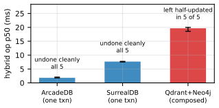
One operation writes both stores in turn: the graph database takes the update first, and the vector store gets its copy second. We raise an error in the gap between the two, a gap that exists in any design where two systems acknowledge separately. The composed stack is left half-updated. The graph database has kept a write the vector store never received, the two disagree about the same records from then on, and neither knows anything is wrong.
That damage stays. Nothing goes back to look for it, so the only records that recover are the ones a later write happens to touch. The corruption is partial and silent: you cannot find it by spot-checking a few records. One engine wrapping the same work in one transaction undoes all of it, leaving the counters where the completed operations left them.
We interrupted 200 trials against each system. The composed stack was left half-updated in all 200. Every single engine on the table, each wrapping the work in one transaction, was left half-updated in none. The count matters: with five trials and no failures you cannot rule out a failure rate near one in two, and two hundred puts it under two in a hundred. Before each interruption the two stores are checked and agree exactly, which is what makes a disagreement afterwards mean something.
This is not a criticism of Qdrant or Neo4j. Both do what they are asked, correctly, every time. The gap is between them, and it belongs to any design in which two systems acknowledge separately; the single engines on the table close it by holding all three models under one transaction. Nor does it mean two stores cannot be made to work: a team would add machinery to repair the divergence afterwards, replaying the missing write until both sides agree. The experiment measures what that machinery buys you, because one engine with one transaction does not need it.
The cross-model operation: a vector hit expands over graph edges and updates a document. ArcadeDB, SurrealDB, Neo4j, and PostgreSQL + pgvector + AGE each do it in one transaction; the composed stack has no transaction spanning its two engines.
| Engine | Mode | Size | p50 ms ↓ | p99 ms ↓ | ingest+index vertices+edges/s ↑ | ingest+index total s ↓ | peak memory GiB ↓ | disk GiB ↓ |
|---|---|---|---|---|---|---|---|---|
| ArcadeDB (one transaction) | embedded | 50k products | 2.03 | 5.77 | 19k | 10.4 | 1.92 | 0.038 |
| ArcadeDB (one transaction) | server | 50k products | 8.87 | 13.2 | 14k | 13.9 | 4.05 | 0.099 |
| ArangoDB | server | 50k products | 5.25 | 7.09 | 43k | 4.63 | 0.57 | 0.14 |
| Neo4j (vector index) | server | 50k products | 17.9 | 28 | 14k | 14.6 | 6.82 | 0.019 |
| PostgreSQL + pgvector + AGE | server | 50k products | 9.05 | 15.2 | 2,320 | 86.2 | 0.11 | 0.16 |
| Qdrant + Neo4j (no shared transaction) | server | 50k products | 20.7 | 36.0 | 34k | 5.93 | 6.81 | 0.0098 |
| SurrealDB | embedded | 50k products | 8.29 | 9.63 | 629 | 318.2 | 0.82 | 0.24 |
| SurrealDB | server | 50k products | 16.1 | 24.2 | 16k | 12.2 | 0.91 | 0.48 |
↑ higher is better, ↓ lower is better; the best value in each column, within one size, is bold
Measured rows: benchmarks/experiments/results/runs_paper.csv
Exact builds measured
- arcadedb 26.9.1-dev · 8d6af9475 (in-process)
- arcadedb 26.9.1-dev · 8d6af9475
arcadedb-c25:8d6af9475 - arangodb 3.12.11
arangodb@563cb2c07af0… - neo4j 2026.07.1
neo4j@1ee8f6fa220f… - PostgreSQL 17.11 + pgvector 0.8.6 + age 1.7.0
dbbench:pg-age - qdrant 1.19.0 + neo4j 2026.07.1
neo4j@1ee8f6fa220f… - surrealdb 2.3.10
- surrealdb 3.2.4
surrealdb/surrealdb@6a5002363ff5…
- Atomic means all or nothing: the whole update happens, or none of it does, with no state in between that anyone can observe. One engine can promise that across a vector, a graph edge, and a document because they share a transaction. Qdrant and Neo4j cannot promise it to each other, because nothing spans the two.
- So the interesting result here is not the speed. It is what a crash halfway through leaves behind. The raw data records, for each run, whether an interrupted write left the two stores disagreeing, and whether they still disagreed after restarting. That is what this comparison exists to show.
- Read the times with one caveat, which cuts against ArcadeDB. Every engine on this table writes to disk except the composed stack's vector half: Qdrant runs in memory (:memory:), so part of why the composed stack's queries answer as they do is that half of it never touches a disk. The all-or-nothing result above does not depend on this, since a half-finished update is visible in memory just as it is on disk, but the millisecond columns do.
- Because the composed stack's Qdrant half runs in memory, its disk value is Neo4j's alone. SurrealDB embedded runs on the SDK's SurrealKV store on disk and SurrealDB server on RocksDB, and each has its own disk reading.
- Disk is what the workload left on disk, in GiB: the engine's writable layer plus its volumes after the cell, minus the same engine's empty footprint.
- The two SurrealDB rows are not one engine in two deployments. The embedded arm runs the core its Python driver carries and the served arm runs the released server, and here those are surrealdb 2.3.10 and surrealdb 3.2.4 -- different versions on different storage engines, released about a year apart. Read each row against the other engines on the table rather than against each other: the distance between these two is not the cost of a network hop.
- ArcadeDB (one transaction), ArcadeDB (server, one transaction), Neo4j (vector index) and Qdrant + Neo4j (no shared transaction) run on a JVM, and for them this column is close to the heap they were given rather than the memory the work needed: Neo4j (vector index)'s 6.82 GiB here is about 114 per cent of its 6g heap, and across every heap this page has run the peak lands between about two thirds of the heap and a fifth above it. Every engine on a table gets the same memory envelope; how much of it a JVM takes is a property of the runtime, so read these cells against each other rather than against an engine that manages its own memory.
- Each repetition runs the transaction 300 times; the p50 and p99 are over those.
- Indexes on this table are matched by effect rather than by rule: ArangoDB, ArcadeDB (one transaction), ArcadeDB (server, one transaction), MongoDB, Neo4j (vector index), PostgreSQL + pgvector + AGE, Qdrant + Neo4j (no shared transaction), SurrealDB (embedded) and SurrealDB (server) build one. Where building one was a choice, the engine was timed with it and without it and the faster configuration kept; where an engine reaches these queries through its own primary key or record id, that is its equivalent. The time an index took to build is the index column.
- ingest+index total s is one timer around loading the vertices and edges and creating the vector index. Ingest paths: ArcadeDB embedded loads with the Python package's graph_batch (5,000 records per commit, vertices then edges) and then CREATE INDEX ... LSM_VECTOR; served sends CREATE VERTEX and CREATE EDGE batches as sqlscript over HTTP, then the same CREATE INDEX; SurrealDB embedded inserts through its Python SDK into the SDK's SurrealKV store on disk, and SurrealDB server through the same SDK over WebSocket onto RocksDB; the composed stack upserts vectors into Qdrant and loads the graph into Neo4j with UNWIND.
The same operation interrupted mid-way, 40 trials per run over five runs. The composed stack is left torn in 40 of 40 trials; every single engine, ArcadeDB embedded and server, SurrealDB embedded and server, Neo4j with its vector index, and PostgreSQL + pgvector + AGE, in 0 of 40, because the whole operation is one transaction that commits or does not.
| Engine | Mode | Size | trials | torn results ↓ |
|---|---|---|---|---|
| ArcadeDB (one transaction) | embedded | 50k products | 40 | 0 |
| ArcadeDB (one transaction) | server | 50k products | 40 | 0 |
| ArangoDB | server | 50k products | 40 | 0 |
| Neo4j (vector index) | server | 50k products | 40 | 0 |
| PostgreSQL + pgvector + AGE | server | 50k products | 40 | 0 |
| Qdrant + Neo4j (no shared transaction) | server | 50k products | 40 | 40 |
| SurrealDB | embedded | 50k products | 40 | 0 |
| SurrealDB | server | 50k products | 40 | 0 |
↑ higher is better, ↓ lower is better; the best value in each column, within one size, is bold
Measured rows: benchmarks/experiments/results/runs_paper.csv
Exact builds measured
- arcadedb 26.9.1-dev · 8d6af9475 (in-process)
- arcadedb 26.9.1-dev · 8d6af9475
arcadedb-c25:8d6af9475 - arangodb 3.12.11
arangodb@563cb2c07af0… - neo4j 2026.07.1
neo4j@1ee8f6fa220f… - PostgreSQL 17.11 + pgvector 0.8.6 + age 1.7.0
dbbench:pg-age - qdrant 1.19.0 + neo4j 2026.07.1
neo4j@1ee8f6fa220f… - surrealdb 2.3.10
- surrealdb 3.2.4
surrealdb/surrealdb@6a5002363ff5…
- A trial writes the three products, kills the process between them, reopens, and checks whether every product is present or none. Torn means some but not all: the counts the page's E2 prose quotes are these.
- The two SurrealDB rows are not one engine in two deployments. The embedded arm runs the core its Python driver carries and the served arm runs the released server, and here those are surrealdb 2.3.10 and surrealdb 3.2.4 -- different versions on different storage engines, released about a year apart. Read each row against the other engines on the table rather than against each other: the distance between these two is not the cost of a network hop.
Benchmarks
Every metric on this page in one figure.
Every metric above appears here as a ratio against the strongest comparator on that row, first pass and repeat pass side by side. Rows follow this page: documents, graph, vectors, time series, and the cross-model transaction, each table in the order shown above and its columns in order, ingest included.
A row marked first pass only has no bar on the right because it is measured once: ingest, writes, transactions, and the 100k sparse tier have no repeat over a warm index, which is defined only for reads. A row marked comparator below resolution has a comparator latency recorded to too few decimals for a ratio.
Each row picks its comparator on the first pass, the fastest engine or the highest throughput, and on the vector rows the fastest engine whose recall is at least ArcadeDB's; the same engine is then read on the repeat pass. At ten million vectors that is 8.75 ms for ArcadeDB against Qdrant's 1.26 and Chroma's 0.70. The dense bar divides by Qdrant rather than Chroma, which the table shows is faster, because Chroma returns 93.4% of the true neighbours where ArcadeDB returns 95.3%.
The repeat pass matters most for ArcadeDB: run the same queries again and ArcadeDB answers in 1.04 ms, because it pages its index off disk and the second pass finds it resident, while Qdrant moves to 1.25 and Chroma to 0.72. So the dense rows flip between the panels, a 1.2x win, with the comparators where they were. The graph rows move too, in both directions, because Neo4j and LadybugDB gain on a repeat pass as well.
On the first pass ArcadeDB wins the OLTP, write, and cross-model rows, matches DuckDB on time-series ingest, and loses every scan-, bulk-, and search-bound row, vector search included. The cross-model row is measured against SurrealDB embedded, the fastest of the single engines here that also do the whole operation in one transaction, rather than the composed stack, which is slower and has no transaction spanning its two engines. Each row uses the comparator's own language: document OLTP is SQL against PostgreSQL, the graph rows are Cypher against LadybugDB or Neo4j, and TPC-H is SQL against DuckDB.

Embedded
The engine as a Python package.
ArcadeDB is a Java engine, and that is friction for Python work: a separate runtime to install, a service to start, and a network hop between your code and your data. The Python package removes all three. It ships the upstream engine unmodified, with a bundled Java runtime and platform wheels, so uv add arcadedb-embedded or pip install arcadedb-embedded is the whole setup and the database runs inside your process.
It is a full API, not a launcher. Transactions and lifecycle, schema and graph helpers, bulk ingest, import and export, and the vector features are all exposed and tested, with the example suite run in CI on every change.
The engine and the Python package are maintained together. Fixes and features found through the benchmarks above are filed and, where possible, contributed upstream. Both are Apache-2.0, and both maintainers, Arcade Data for the engine and HumemAI for this package, have said they will keep it that way.
What does the Python boundary cost? The engine runs at the same speed either way; what you pay for is handing results back. Against Java in the same process doing the same work, a vector search costs 1.04x and a 100k-document scan 1.75x.
The bigger number is inside Python. Asking for record objects is 15.1x slower than asking for columns over the same query, so which call you use, to_list or to_columns, matters more than the language boundary does. Check that before blaming the engine for a slow loop.
The same query answered from Java and from Python, and the three ways Python can ask for the results: `to_columns`, `to_json_list`, and `to_list`.
| Engine | Size | time ms ↓ | vs Java ↓ |
|---|---|---|---|
| Java, in process | vector search | 1.52 | 1.00x |
| Python | vector search | 1.58 | 1.04x |
| Java, in process | 100k-document scan | 145.3 | 1.00x |
| Python, to_columns | 100k-document scan | 254.6 | 1.75x |
| Python, to_json_list | 100k-document scan | 384.0 | 2.64x |
| Python, to_list | 100k-document scan | 3,857 | 26.6x |
↑ higher is better, ↓ lower is better; the best value in each column, within one size, is bold
Measured rows: benchmarks/python-bindings/jpype_overhead/results/mini_results.csv
- The engine itself runs at the same speed either way. What Python is charged for is moving results across the boundary, which is why the vector search costs 1.04x and the scan 1.75x rather than anything scaling with the work the engine did.
- The path you choose inside Python matters far more than the language boundary does. Asking for record objects is 15.1x slower than asking for columns over the same query, so the practical advice is to use the columnar or batched call for anything large.
Starting the engine is the other cost, and it is paid once per process, not per query. A cold process reaches its first database call in about 0.45 s, most of it the Java runtime starting; after that, opening and closing an empty database costs about 4.4 ms. The table below is one session each, open, do one thing, close, for every kind of data at four sizes, embedded and against the server.
Session cost by kind of data and size, embedded and against the server. The dense-vector rows at 1M and 10M show an engine defect, the first query after a write waited on a full index rebuild; it is filed as #7183, fixed upstream for 26.10.1, and a later campaign re-measures it.
| Engine | Mode | Size | JVM start ms ↓ | first open ms ↓ | cold process ms ↓ | open and close ms ↓ | one query ms ↓ | one write ms ↓ | write, then query ms ↓ | peak memory GiB ↓ |
|---|---|---|---|---|---|---|---|---|---|---|
| Dense vectors | embedded | 10k | 185.0 | 201.9 | 506.5 | 8.41 | 23.3 | 18.8 | 555.8 | 2.73 |
| Dense vectors | server | 10k | — | — | — | 9.65 | 36.5 | 21.2 | 559.3 | 1.87 |
| Documents | embedded | 10k | 178.1 | 151.5 | 439.7 | 4.74 | 5.27 | 13.8 | 13.3 | 0.35 |
| Documents | server | 10k | — | — | — | 7.41 | 9.52 | 17.4 | 19.2 | 0.37 |
| Documents, ten indexes | embedded | 10k | 180.1 | 167.1 | 466.5 | 11.0 | 11.8 | 40.1 | 39.5 | 0.78 |
| Documents, ten indexes | server | 10k | — | — | — | 17.4 | 17.7 | 75.9 | 71.2 | 0.79 |
| Empty database | embedded | 10k | 181.6 | 156.1 | 449.3 | 4.44 | 4.24 | 13.4 | 13.2 | 0.25 |
| Empty database | server | 10k | — | — | — | 6.96 | 6.90 | 15.7 | 17.3 | 0.30 |
| Graph | embedded | 10k | 191.7 | 160.1 | 465.9 | 6.48 | 8.61 | 13.9 | 13.9 | 2.05 |
| Graph | server | 10k | — | — | — | 8.60 | 12.5 | 17.9 | 18.8 | 2.08 |
| Sparse vectors | embedded | 10k | 181.2 | 164.0 | 458.7 | 5.31 | 5.84 | 25.2 | 25.2 | 1.04 |
| Sparse vectors | server | 10k | — | — | — | 7.72 | 11.1 | 30.9 | 28.7 | 1.16 |
| Time series | embedded | 10k | 179.8 | 170.8 | 475.8 | 18.9 | 11.2 | 23.8 | 22.2 | 2.00 |
| Time series | server | 10k | — | — | — | 12.7 | 14.8 | 23.8 | 24.5 | 1.96 |
| Dense vectors | embedded | 100k | 183.6 | 206.2 | 503.4 | 16.7 | 100.0 | 24.2 | 207.6 | 2.94 |
| Dense vectors | server | 100k | — | — | — | 10.5 | 114.6 | 27.7 | 211.9 | 4.22 |
| Documents | embedded | 100k | 184.7 | 156.0 | 447.9 | 4.62 | 4.86 | 12.5 | 14.0 | 0.83 |
| Documents | server | 100k | — | — | — | 6.63 | 9.14 | 16.1 | 18.4 | 0.91 |
| Documents, ten indexes | embedded | 100k | 184.8 | 168.8 | 470.9 | 11.0 | 11.2 | 38.9 | 38.7 | 2.66 |
| Documents, ten indexes | server | 100k | — | — | — | 24.0 | 21.8 | 41.7 | 44.5 | 2.09 |
| Empty database | embedded | 100k | 185.3 | 155.0 | 460.8 | 4.23 | 4.24 | 13.5 | 13.8 | 0.24 |
| Empty database | server | 100k | — | — | — | 7.56 | 7.35 | 15.5 | 15.5 | 0.29 |
| Graph | embedded | 100k | 181.2 | 159.5 | 456.1 | 5.92 | 8.71 | 13.3 | 14.2 | 2.76 |
| Graph | server | 100k | — | — | — | 8.18 | 11.2 | 16.4 | 18.7 | 2.75 |
| Sparse vectors | embedded | 100k | 181.2 | 159.5 | 447.7 | 5.43 | 6.09 | 21.0 | 18.7 | 2.73 |
| Sparse vectors | server | 100k | — | — | — | 7.54 | 9.90 | 27.5 | 27.7 | 4.12 |
| Time series | embedded | 100k | 180.4 | 168.0 | 481.7 | 10.6 | 10.5 | 21.4 | 20.5 | 2.69 |
| Time series | server | 100k | — | — | — | 11.9 | 15.1 | 20.6 | 25.9 | 2.67 |
| Dense vectors | embedded | 1M | 185.2 | 194.3 | 496.7 | 98.4 | 878.6 | 94.1 | 1,810 | 12.8 |
| Dense vectors | server | 1M | — | — | — | 11.4 | 919.3 | 102.8 | 2,043 | 12.7 |
| Documents | embedded | 1M | 182.9 | 146.9 | 435.5 | 4.65 | 4.95 | 14.1 | 13.9 | 4.69 |
| Documents | server | 1M | — | — | — | 6.10 | 7.91 | 15.3 | 18.3 | 4.44 |
| Documents, ten indexes | embedded | 1M | 181 | 172.4 | 476.2 | 22.3 | 23.1 | 56.6 | 55.9 | 10.4 |
| Documents, ten indexes | server | 1M | — | — | — | 22.9 | 33.3 | 87.2 | 65.9 | 10.4 |
| Empty database | embedded | 1M | 182.0 | 153.4 | 440.7 | 5.35 | 5.38 | 14.4 | 13.5 | 0.47 |
| Empty database | server | 1M | — | — | — | 8.15 | 7.15 | 18.0 | 17.6 | 0.52 |
| Graph | embedded | 1M | 178.2 | 146.0 | 433.5 | 5.79 | 9.07 | 12.1 | 14.1 | 10.5 |
| Graph | server | 1M | — | — | — | 7.82 | 10.4 | 18.5 | 18.4 | 10.5 |
| Sparse vectors | embedded | 1M | 178.4 | 155.0 | 440.3 | 5.29 | 6.18 | 22.4 | 22.9 | 10.5 |
| Sparse vectors | server | 1M | — | — | — | 7.23 | 13.0 | 27.1 | 26.1 | 10.5 |
| Time series | embedded | 1M | 187.1 | 165.2 | 471.9 | 10.5 | 10.5 | 20.7 | 17.4 | 10.1 |
| Time series | server | 1M | — | — | — | 12.8 | 14.7 | 21.3 | 23.9 | 10.1 |
| Dense vectors | embedded | 10M | 187.9 | 193.2 | 493.8 | 1,420 | 18k | 1,488 | 18k | 24.7 |
| Dense vectors | server | 10M | — | — | — | 20.4 | 18k | 1,491 | 18k | 24.7 |
| Documents | embedded | 10M | 180.5 | 144.4 | 428.6 | 5.06 | 5.30 | 14.0 | 13.4 | 15.3 |
| Documents | server | 10M | — | — | — | 6.07 | 7.65 | 13.9 | 15.8 | 15.3 |
| Time series | embedded | 10M | 186.0 | 172.5 | 477.6 | 10.5 | 11.2 | 22.3 | 19.7 | 15.2 |
| Time series | server | 10M | — | — | — | 13.5 | 14.8 | 26.6 | 22.6 | 15.3 |
↑ higher is better, ↓ lower is better; the best value in each column, within one size, is bold
Measured rows: benchmarks/experiments/results/runs_paper.csv
- The SESSION is open + action + close. Reporting open and close alone hides work triggered between them.
- Cold start is measured in a fresh subprocess and reported beside every session number, because a millisecond open inside a process that takes half a second to reach its first database call is not a millisecond to whoever launched it.
- Known at this engine build: a vector database's no-op session close grows with the index (8 ms at 10k, 98 ms at 1M, 1.4 s at 10M), and a session with one search in it at 10M is 17.6 s, because the first search after a write started a full asynchronous graph rebuild and close() waited on it. Filed as #7183, fixed upstream in #7191 for 26.10.1; the October re-pin re-measures it.
- A clean close should be O(what was written), not O(what is stored): write nothing and closing should cost the same at 10k documents and 10M.
- Server rows have no JVM start, first open, or cold process: the server is already running when the probe connects, so those three columns describe the embedded process only. The session columns are measured for both.
- Graph with the analytical view is withheld: its query grew from a bounded set of seeds to an unbounded 2-hop, so the cell is re-measured in October
Embedded or server is the deployment choice, and the tables above run the same engine build in both, so the difference between them is the deployment and not the engine. SurrealDB also has both modes, and its two rows above sit far apart: its Python package embeds a core a major version behind its server, on a different storage engine, so the embedded row wins only the point lookups the wire would have cost and loses or times out on every bulk cell. ArcadeDB's engine and Python package are released together from the same build, so that gap does not exist here.
Running the database in a separate process costs two things added together: turning the answer into a wire format that can travel over a connection, and the connection itself. The table below separates them by measuring a third deployment in between, an HTTP server running inside the same process. Embedded to that middle deployment adds the wire format without a second process. The middle deployment to a separate container adds the second process without changing the wire format.
The same projection answered by three deployments at six result sizes. The first column to the second is the wire format; the second to the third is the process boundary.
| Engine | Size | in-process ms ↓ | in-process server, HTTP ms ↓ | separate container, HTTP ms ↓ |
|---|---|---|---|---|
| 1 documents | 1 | 1.26 | 2.58 | 2.89 |
| 10 documents | 10 | 0.96 | 1.97 | 2.16 |
| 100 documents | 100 | 1.48 | 3.59 | 4.04 |
| 1,000 documents | 1,000 | 3.35 | 5.27 | 4.56 |
| 10,000 documents | 10,000 | 21.2 | 27.8 | 26.6 |
| 100,000 documents | 100,000 | 207.3 | 241.5 | 252.2 |
↑ higher is better, ↓ lower is better; the best value in each column, within one size, is bold
Measured rows: benchmarks/experiments/results/e4decomp_8d6af9475
Exact builds measured
- arcadedb 26.9.1-dev · 8d6af9475
- Every number is milliseconds. One engine build (arcadedb 26.9.1-dev · 8d6af9475) in all three deployments, 15 repetitions after 3 warmup, identical cpuset 0-11, memory cap 8g and heap 6g.
- All three deployments turn the answer into Python objects the same way, so the difference is how the database was deployed and not how we read the result.
- The separate container runs on the same machine, talking over the local network interface. It says what running the database beside your program costs, and says nothing about a database on another machine across a real network.
- The separate-process column goes slightly negative at the smaller result sizes. That is not a container being faster than an in-process server; it is the boundary term sitting below what this design can resolve, so run-to-run noise swamps it and the sign flips. Reported rather than clamped to zero, because the negative values are the evidence for the claim: at these sizes co-locating costs nothing measurable. The packing cost, in the column beside it, stays firmly positive at every size.
The two are nowhere near equal. The wire format costs something at every size and grows with the result. The process boundary, the second column against the third, is so small that at the smaller sizes it disappears into the noise. So the cost of running client and server as separate processes on one machine is the wire format, not the separation, and the lever that would move it is a cheaper wire format, not co-location.

Use embedded when the database serves one process: notebooks, tests, single-node services, agent tooling, and anything where a network hop per query is pure cost. It installs with pip install, starts in under half a second, and has no service to operate.
Use the server when more than one process or machine needs the same data, when you want the Postgres, Redis, Bolt, or HTTP wire protocols, or when you need Raft replication and failover. The Python package can also start a server inside your process, so you can move from one to the other later.
This is a deployment decision, not a performance one. The engine is the same in both, and the difference you will feel is the boundary you put around it.
Licenses
What each engine's license allows.
Not every engine on this page is open source in the sense the Open Source Initiative (OSI) defines. ArcadeDB and the Python package are both Apache-2.0.
| Engine | License | Any use, free | Your code stays yours |
|---|---|---|---|
| ArcadeDB engine | Apache-2.0 | yes | yes |
| arcadedb-embedded (the Python package) | Apache-2.0 | yes | yes |
| PostgreSQL and pgvector | PostgreSQL License | yes | yes |
| Apache AGE | Apache-2.0 | yes | yes |
| DuckDB | MIT | yes | yes |
| SQLite | public domain | yes | yes |
| sqlite-vec | Apache-2.0 | yes | yes |
| MongoDB Community | SSPL-1.0 | no | no |
| Neo4j Community | GPL-3.0 (Enterprise is commercial) | yes | no |
| LadybugDB | MIT | yes | yes |
| Qdrant | Apache-2.0 | yes | yes |
| Milvus | Apache-2.0 | yes | yes |
| Elasticsearch | AGPL-3.0 (also SSPL and ELv2) | yes | no |
| Chroma | Apache-2.0 | yes | yes |
| LanceDB | Apache-2.0 | yes | yes |
| QuestDB | Apache-2.0 | yes | yes |
| TimescaleDB | Timescale License (the image used here); the core alone is Apache-2.0 | no | no |
| SurrealDB | Business Source License 1.1 | no | no |
| ArangoDB | Business Source License 1.1 | no | no |
Two tests, each answered from the license text at the pinned version in September 2026. Any use, free: anyone may run the engine for any purpose, including selling a product or a service built on it, without paying the vendor; the SSPL (MongoDB), the Business Source License (SurrealDB and ArangoDB), and the Timescale License (the TimescaleDB image used here; its core alone is Apache-2.0) all reserve some uses. Your code stays yours: you may modify the engine and ship or serve a product on it without publishing your own code; the GPL (Neo4j Community) and the AGPL (Elasticsearch, whose core is offered under a choice of three licenses since 2024 and whose sparse-vector search measured here is in that core) require sharing what you distribute or serve. Rows in bold pass both tests. Both tests are yes for permissive licenses (Apache-2.0, MIT, the PostgreSQL License) and the public domain, yes and no for copyleft, and no for source-available. The Open Source Initiative approves every license in the first two groups and none in the third. A license can change with a release.
Four engines on this page are single-stack multi-model databases, one process serving documents, graph, and vectors: ArcadeDB, ArangoDB, MongoDB, and SurrealDB. Among them ArcadeDB is the only one that passes both tests above, Apache-2.0 since its first commit in 2021, and the only one whose engine and Python bindings ship together in monthly releases; MongoDB moved from the AGPL to the SSPL in 2018, ArangoDB from Apache-2.0 to the Business Source License in 2024, and SurrealDB has used the Business Source License since its public release. On staying that way, ArcadeDB's founder wrote in February 2026 that the project will never change its license; this page reports that as his published statement, not as a guarantee. HumemAI, which maintains arcadedb-embedded, makes the same commitment for the Python package: the engine and its bindings both stay Apache-2.0. PostgreSQL with pgvector and AGE reaches the same one-transaction result by loading extensions into one process, and it is open source under both tests; it is not counted among the four because three projects maintain its three models.
Resources